HW 9 Solutions
ENGR 21, Fall 2026.
Solutions
1 Pivoting
1.1 By hand
Consider the matrix \[A = \begin{bmatrix} 0 & 2 & 5 & -1 \\ 2 & 1 & 3 & 0 \\ -2 & -1 & 4 & 1 \\ 3 & 7 & -1 & 2 \\ \end{bmatrix}\]
If this matrix is decomposed into \(L\) and \(U\) following Doolittle’s factorization, determine the upper triangular matrix \(U\), showing all intermediate stages of the matrix in the Gaussian elimination procedure and describing what each step accomplishes.
- Starting work on column 1. Swap rows 1 and 2
\[ \begin{bmatrix} 2 & 1 & 3 & 0 \\ 0 & 2 & 5 & -1 \\ -2 & -1 & 4 & 1 \\ 3 & 7 & -1 & 2 \\ \end{bmatrix} \]
- No need to eliminate \(A_{21}\). Eliminating \(A_{31}\):
\[ \begin{bmatrix} 2 & 1 & 3 & 0 \\ 0 & 2 & 5 & -1 \\ 0 & 0 & 7 & 1 \\ 3 & 7 & -1 & 2 \\ \end{bmatrix} \]
- Eliminating \(A_{41}\):
\[ \begin{bmatrix} 2 & 1 & 3 & 0 \\ 0 & 2 & 5 & -1 \\ 0 & 0 & 7 & 1 \\ 0 & 5.5 & -5.5 & 2 \\ \end{bmatrix} \]
- Starting work on column 2. Swap rows 2 and 4:
\[ \begin{bmatrix} 2 & 1 & 3 & 0 \\ 0 & 5.5 & -5.5 & 2 \\ 0 & 0 & 7 & 1 \\ 0 & 2 & 5 & -1 \\ \end{bmatrix} \]
- No need to eliminate \(A_{32}\). Eliminating \(A_{42}\):
\[ \begin{bmatrix} 2 & 1 & 3 & 0 \\ 0 & 5.5 & -5.5 & 2 \\ 0 & 0 & 7 & 1 \\ 0 & 0 & 7 & -1.727 \\ \end{bmatrix} \]
- Starting work on column 3. No swapping necessary. Eliminating \(A_{43}\):
\[ \begin{bmatrix} 2 & 1 & 3 & 0 \\ 0 & 5.5 & -5.5 & 2 \\ 0 & 0 & 7 & 1 \\ 0 & 0 & 0 & -2.727 \\ \end{bmatrix} \]
Therefore, the final result is \[ \begin{bmatrix} 2 & 1 & 3 & 0 \\ 0 & 5.5 & -5.5 & 2 \\ 0 & 0 & 7 & 1 \\ 0 & 0 & 0 & -2.727 \\ \end{bmatrix} \]
1.2 Python program for pivoting
Write a Python function named eliminate_pivot that takes as input a single matrix and performs Gaussian elimination with pivoting on that matrix.
def eliminate_pivot(A):
    n = len(A)
    scale_rows = np.zeros(n)
    for k in range(0,n-1):
        # Determine the scale factor of each row
        for i in range(n):
            scale_rows[i] = max(abs(A[i,:]))
        # Re-calculate relative sizes.
        relative_sizes = abs(A[k:,k])/scale_rows[k:]

        # Look for the best row
        best_row = np.argmax(relative_sizes)

        if best_row+k != k:
            A = swap_rows(A,k,best_row+k)

        # Gauss elimination
        for i in range(k+1,n):
            # Row i = Row i - multiplier * Row k
            A[i,:] = A[i,:] - (A[i,k]/A[k,k])*A[k,:]
    return A
2 The Jacobi Algorithm
Jacobi with while loop
In lecture, we have seen an algorithm for Jacobi’s method that carries out n_steps iterations in a for loop. Write a Python function named Jacobi that instead makes use of a while loop, terminating the iterations when the norm of the residual is less than tol.
Your function should take as input the following quantities in order: \(A\), the system matrix; \(b\), the right-hand-side vector; \(x^{(0)}\), the first guess for \(x\), and tol, a tolerance parameter that is typically set to a very small number such as \(10^{-6}\). The function should return the most recent vector \(x^{(k)}\).
You can use b - numpy.dot(A,x) to calculate the vector \(b - Ax\).
def Jacobi(A,b,x0,tol):
    normres = 1 # Start with a dummy value
    xold = x0
    xnew = np.zeros(np.shape(xold))
    while normres > tol:
        for j in range(len(xold)):
            total = 0
            for i in range(len(xold)):
                if i != j:
                    total += A[j,i] * xold[i]
            xnew[j] = (1/(A[j,j])) * (b[j] - total)
        # Calculate residual
        residual = b - np.dot(A,xnew)
        normres = norm(residual)

        print(xnew," and |res| = ",normres)
        xold = xnew.copy()
    return xnew
3 Gauss-Seidel
As we saw in lecture 17, the Gauss-Seidel algorithm modifies the Jacobi algorithm so that it makes use of the new \(x\) values as they are computed. The first row’s update is based entirely on the old values; the second row’s update is based on the old values for \(x_3\), \(x_4\), …, \(x_n\), but it makes use of the newly-computed value for \(x_{1}\); the third row’s update is based on the old values for \(x_4\), \(x_5\), …, \(x_n\), but it makes use of the newly-computed value for \(x_{1}\) and \(x_2\).
3.1 Python code
Write a Python function named GaussSeidel that carries out a specified number of iterations of the Gauss-Seidel algorithm.
Your function should take as input the following quantities in order: \(A\), the system matrix; \(b\), the right-hand-side vector; \(x^{(0)}\), the first guess for \(x\), and \(n\), the number of iterations. The function should return the most recent vector \(x^{(k)}\).
3.2 Gauss-Seidel vs Jacobi
You will solve the same equation \(Ax=b\) iteratively using the two iterative methods, Gauss-Seidel and Jacobi. You are welcome to use a computer to help you with this problem, but your answers should be written out by hand.
Solve the system of equations represented by the augmented matrix
\[ \left[ \begin{array}{ccc|c} 6 & 3 & 1 & 1 \\ 2 & 7 & 4 & 0 \\ 5 & 1 & 8 & 0 \end{array} \right] \]
starting with the guess \(x_1 = 1, x_2 = 0, x_3 = 2\) using:
- Two iterations of the Gauss-Seidel algorithm, and
- Two iterations of the Jacobi algorithm.
For each iteration, show all your work, and also calculate and write down the norm of the residual vector at the end of each iteration.
Gauss-Seidel, using the new values of \(x\) as soon as they are available.
\(x^{(0)} = [1, 0, 2]\).
\[ \begin{align} x^{(1)}_1 &= \frac{1}{6} \left( 1 - 3 \times 0 - 1 \times 2\right) = -\frac{1}{6} \approx -0.167 \\ x^{(1)}_2 &= \frac{1}{7} \left( 0- 2 \times \left( -\frac{1}{6} \right) - 4 \times 2 \right) = -\frac{23}{21} \approx -1.095 \\ x^{(1)}_3 &= \frac{1}{8} \left( 0 - 5 \times \left( -\frac{1}{6}\right) - 1 \times \left( -\frac{23}{21}\right) \right) = \frac{81}{336} \approx 0.241 \end{align} \]
At this stage, \(x^{(1)} = [-0.1667, -1.095, 0.2410]\) and the residual vector is \[b - Ax = \begin{bmatrix} 1 \\ 0 \\ 0 \end{bmatrix} - \begin{bmatrix} 6 & 3 & 1 \\ 2 & 7 & 4 \\ 5 & 1 & 8 \end{bmatrix} \begin{bmatrix} -0.1667 \\ -1.095 \\ 0.2410 \end{bmatrix} = \begin{bmatrix} 5.0446 \\ 7.0357 \\ 0 \end{bmatrix}\]
and the norm of this vector is \(\boxed{8.65}\).
Then, we do this again:
\[ \begin{align} x^{(2)}_1 &= \frac{1}{6} \left( 1 - 3 \times \left( -\frac{23}{21}\right) - 1 \times \left( \frac{81}{336} \right) \right) \approx 0.674 \\ x^{(2)}_2 &= \frac{1}{7} \left( 0- 2 \times \left( 0.674 \right) - 4 \times \left( \frac{81}{336} \right) \right) \approx -0.3303 \\ x^{(2)}_3 &= \frac{1}{8} \left( 0 - 5 \times \left( 0.674 \right) - 1 \times \left( -0.3303 \right) \right) \approx -0.3800 \end{align} \]
At this stage, \(x^{(2)} = [ 0.674, -0.3303, -0.3800]\) and the residual vector is \[b - Ax = \begin{bmatrix} 1 \\ 0 \\ 0 \end{bmatrix} - \begin{bmatrix} 6 & 3 & 1 \\ 2 & 7 & 4 \\ 5 & 1 & 8 \end{bmatrix} \begin{bmatrix} 0.674 \\ -0.3303 \\ -0.3800 \end{bmatrix} = \begin{bmatrix} -1.673 \\ 2.484 \\ \approx 0 \end{bmatrix}\]
and the norm of this vector is \(\boxed{2.995}\).
Jacobi, avoids using newly-calculated values of \(x\) as soon as they are available, and instead waits for the new iteration before it updates.
\(x^{(0)} = [1, 0, 2]\).
\[ \begin{align} x^{(1)}_1 &= \frac{1}{6} \left( 1 - 3 \times 0 - 1 \times 2\right) = -\frac{1}{6} \approx -0.167 \\ x^{(1)}_2 &= \frac{1}{7} \left( 0- 2 \times 1 - 4 \times 2 \right) = -\frac{10}{7} \approx -1.428 \\ x^{(1)}_3 &= \frac{1}{8} \left( 0 - 5 \times 1 - 1 \times 0 \right) = -\frac{5}{8} = -0.625 \end{align} \]
At this stage, \(x^{(1)} = [-0.167, -1.428, -0.625]\) and the residual vector is \[b - Ax = \begin{bmatrix} 1 \\ 0 \\ 0 \end{bmatrix} - \begin{bmatrix} 6 & 3 & 1 \\ 2 & 7 & 4 \\ 5 & 1 & 8 \end{bmatrix} \begin{bmatrix} -0.167 \\ -1.428 \\ -0.625 \end{bmatrix} = \begin{bmatrix} 6.910 \\ 12.833 \\ 7.261 \end{bmatrix}\]
and the norm of this vector is \(\boxed{16.28}\).
Then, we do this again:
\[ \begin{align} x^{(2)}_1 &= \frac{1}{6} \left( 1 - 3 \times \left( - \frac{10}{7} \right) - 1 \times \left( - \frac{5}{8} \right) \right) \approx 0.985 \\ x^{(2)}_2 &= \frac{1}{7} \left( 0- 2 \times \left( -\frac{1}{6} \right) - 4 \times \left( - \frac{5}{8} \right) \right) \approx 0.4047 \\ x^{(2)}_3 &= \frac{1}{8} \left( 0 - 5 \times \left( -\frac{1}{6} \right) - 1 \times \left( -\frac{10}{7}\right) \right) \approx 0.2827 \end{align} \]
At this stage, \(x^{(2)} = [0.985, 0.4047, 0.2827]\) and the residual vector is \[b - Ax = \begin{bmatrix} 1 \\ 0 \\ 0 \end{bmatrix} - \begin{bmatrix} 6 & 3 & 1 \\ 2 & 7 & 4 \\ 5 & 1 & 8 \end{bmatrix} \begin{bmatrix} 0.985 \\ 0.4047 \\ 0.2827 \end{bmatrix} = \begin{bmatrix} -6.407 \\ -5.934 \\ -7.592 \end{bmatrix}\]
and the norm of this vector is \(\boxed{11.57}\).
4 Convergence of Iterative Methods
The norm of the residual vector after each iteration gives us information about how close to the true solution a numerical method gets after \(n\) iterations. In this problem, you will examine this for a simple 3x3 system (which could easily be solved exactly by direct methods) to illustrate the convergence properties of the Jacobi and Gauss-Seidel algorithms.
In practice, engineers need to solve systems of equations that have thousands or millions of rows, and the speed with which a numerical method can get close to the right answer becomes extremely important.
For the system represented by the augmented matrix \[ \left[ \begin{array}{ccc|c} 6 & 3 & 1 & 1 \\ 2 & 7 & 4 & 0 \\ 5 & 1 & 8 & 0 \end{array} \right], \]
starting from the guess \([1,0,2]\),
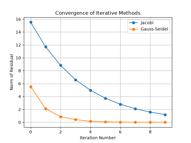
- Make a plot of the norm of the residual vector after 10 iterations of the Gauss-Seidel method and of the Jacobi method.
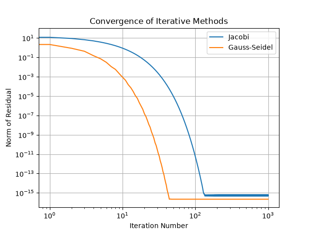
- Make a plot of the norm of the residual vector after 1,000 iterations of the two methods on a log-log scale. Use
matplotlib.pyplot.xscale("log")andmatplotlib.pyplot.yscale("log"). - Describe and explain what these graphs tell us. You may wish to look at lecture 8.
You must make your plots in matplotlib and include the code with your submission.
You can download the below as a single file here.
For this problem, both Jacobi and GaussSeidel were defined to take as argument the number of iterations.
Jacobi function:
def Jacobi(A,b,x0,n):
    rhist = np.zeros(n)
    xold = x0
    xnew = np.zeros(np.shape(xold))
    for k in range(n):
        for j in range(len(xold)):
            total = 0
            for i in range(len(xold)):
                if i != j:
                    total += A[j,i] * xold[i]
            xnew[j] = (1/(A[j,j])) * (b[j] - total)
        # Calculate residual
        residual = b - np.dot(A,xnew)
        # Find norm and store
        normres = norm(residual)
        rhist[k] = normres

        xold = xnew.copy()
    return rhist
Gauss-Seidel function:
def GaussSeidel(A,b,x0,n):

    rhist = np.zeros(n)
    x = x0
    for k in range(n):
        for j in range(len(x)):
            total = 0
            for i in range(len(x)):
                if i != j:
                    total += A[j,i] * x[i]
            x[j] = (1/(A[j,j])) * (b[j] - total)
        # Calculate residual
        residual = b - np.dot(A,x)
        # Find norm and store
        normres = norm(residual)
        rhist[k] = normres
    return rhist
Matrix definitions and import statements:
Plotting procedure:
hist_J = Jacobi(A,b,np.array([1,1,1],dtype=np.float64),1000)
hist_G = GaussSeidel(A2,b,np.array([1,1,1],dtype=np.float64),1000)

# Figure 1

plt.plot(np.transpose([hist_J[:10], hist_G[:10]]),'o-',label=['Jacobi','Gauss-Seidel'])
plt.grid(True)
plt.legend()
plt.xlabel("Iteration Number")
plt.ylabel("Norm of Residual")
plt.title("Convergence of Iterative Methods")
plt.savefig("Jacobi-Gauss-1.png")
plt.close()

# Figure 2
plt.plot(np.transpose([hist_J, hist_G]),'-',label=['Jacobi','Gauss-Seidel'])
plt.grid(True)
plt.legend()
plt.xscale("log")
plt.yscale("log")
plt.xlabel("Iteration Number")
plt.ylabel("Norm of Residual")
plt.title("Convergence of Iterative Methods")
plt.savefig("Jacobi-Gauss-1.png")
The resulting graphs are shown below.
Description and explanation
The graphs show that both methods rapidly reduce the residual to nearly zero, but Gauss-Seidel is faster at this than Jacobi. On a log-log scale, the behavior follows a straight line at large \(n\), which means that there is exponential decay of the norm of the residual once about 10 iterations have passed for G-S and once about 50 iterations have passed for Jacobi. Eventually, both methods bring the norm of the residual down to a number that is effectively zero, close to machine epsilon for 64-bit floating point numbers as shown in lecture 8.