Lecture 20
E21 Computer Engineering Fundamentals
Linear & Nonlinear Interpolation
Fitting a polynomial of degree \(n\) to a set of \(n+1\) points is an example of linear interpolation.
Interpolate the polynomial \[y = a_0 + a_1 x + a_2 x^2 + ... a_n x^n \] to the points \(\{ x_0, y_0 \}, \{ x_1, y_1 \}, \{ x_2, y_2 \}, ... , \{ x_n, y_n \}\) by solving an equation for the parameters \(\{ a_0, a_1, a_2, ..., a_n \}\)
\[ {\begin{bmatrix} x_0^0 & x_0^1 & x_0^2 & \cdots & x_0^n \\ x_1^0 & x_1^1 & x_1^2 & \cdots & x_1^n \\ \vdots & \vdots & \vdots & \ddots & \vdots \\ x_n^0 & x_n^1 & x_n^2 & \cdots & x_n^n \end{bmatrix}} \begin{bmatrix} a_0 \\ a_1 \\ \vdots \\ a_n \end{bmatrix} = \begin{bmatrix} y_0 \\ y_1 \\ \vdots \\ y_n \end{bmatrix} \]
What’s nonlinear interpolation ?
Nonlinear interpolation is when the interpolating function depends nonlinearly on the looked-for parameters.
An example of nonlinear interpolation
Interpolate the points \(\{ 0.5, 0.6191\}, \{ 1, 0.24612\}, \{ 2, -0.0277\}\) to the curve \(\boxed{y(x) = a e^{-b x} \sin (c x)}\).
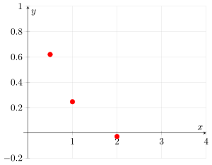
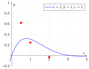
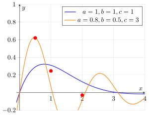
Write down the mathematical equations for this problem.
Equations for nonlinear interpolation
Interpolating \(\{ 0.5, 0.6191\}, \{ 1.0, 0.24612\}, \{ 2.0, -0.0277\}\) to \(\boxed{y(x) = a e^{-b x} \sin (c x)}\)
requires solving three equations for three unknowns
\[ \begin{align*} \phantom{-}0.6191 &= a e^{-b \times 0.5} \sin (c \times 0.5) \\ \phantom{-}0.2461 &= a e^{-b \times 1.0} \sin (c \times 1.0) \\ -0.0277 &= a e^{-b \times 2.0} \sin (c \times 2.0) \end{align*} \]
Notice that the interpolating function \(y(x)\) depends nonlinearly on the parameters \(b\) and \(c\).
i.e., an equation of this kind does not exist:
\[ {\begin{bmatrix} A_{11} & A_{12} & A_{13} \\ A_{21} & A_{22} & A_{23} \\ A_{31} & A_{32} & A_{33} \end{bmatrix}} \begin{bmatrix} a \\ b \\ c \end{bmatrix} = \begin{bmatrix} d_1 \\ d_2 \\ d_3 \end{bmatrix} \]
Successful Interpolation with other-than-polynomial functions
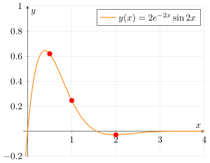
- The function \(y(x) = 2 e^{-2x} \sin 2x\) happens to pass through all three given points exactly.
The need for Curve Fitting
Consider the following data points and make
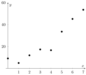
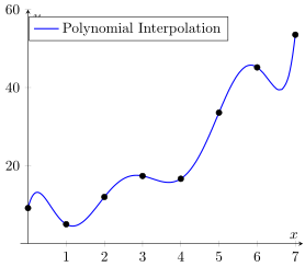
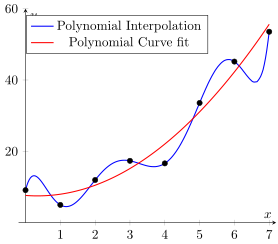
- Polynomial interpolation follows the given data exactly
- But practically, we sometimes just want the trend
- Curve fits are a mathematically-determined ‘curve of best fit’
Line of best fit
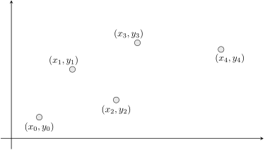
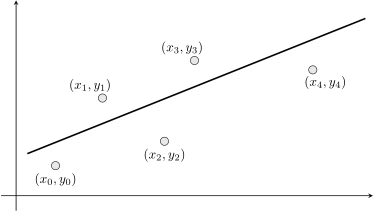
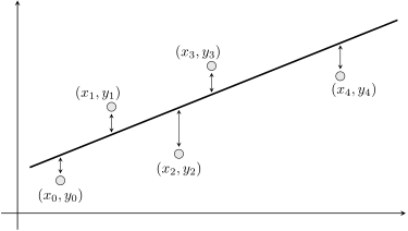
Goal: Find a straight line that is as close as possible to the data points
- Draw any straight line with equation \(y = f(x)\)
- Measure the components of a ‘residual vector’ \(r_i = y_i - f(x_i)\)
- vertical distance between a point and the line of best fit
- Adjust the line until the norm of the residual vector is the smallest it will ever be.
Goal: Find \(f(x) = a_0 + a_1 x\) such that \(\sum r_i^2\) is minimized.
“Minimize the sum of the squares of the residuals”
Least Squares Fit
- A ‘least squares fit’ is much more general than straight lines or even polynomials.
- Potentially, any function can be fit to given data by minimizing the sum of the squares of the residuals
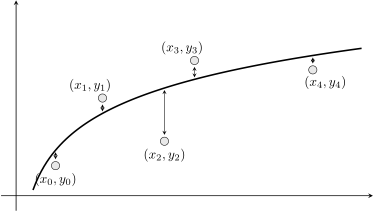
Linear vs. nonlinear least squares
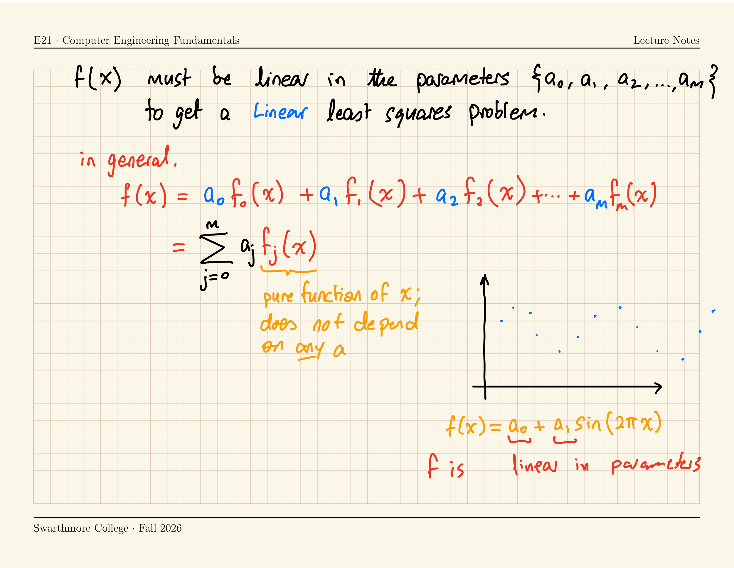
- Consider some functions \(f(x)\) that depend also on some parameters \(\{ a_0, a_1, a_2, ... \}\):
- \(f(x) = a_0 + a_1 \sin x\)
- \(f(x) = a_0 x - \log x\)
- \(f(x) = a_0 x - \log a_1 x\)
- \(f(x) = a_0 x + a_1 \log x\)
- \(f(x) = a_0 x + a_1 x^3 - a_2 x^5\)
- \(f(x) = a_0 \sin (a_1 x) + a_2\)
Which of these is linear in the parameters \(a_i\) and which is nonlinear in the parameters \(a_i\) ?
Linear vs. nonlinear least squares
Linear Least Squares
Function \(f(x)\) depends linearly on the parameters \(\{ a_0, a_1, a_2, ... \}\)
Nonlinear Least Squares
Function \(f(x)\) depends nonlinearly on at least one of the parameters \(\{ a_0, a_1, a_2, ... \}\)
- In both cases, \(f(x)\) is allowed to be nonlinear in \(x\).
Curve Fitting \(n\) data points to \(m\)-degree polynomial
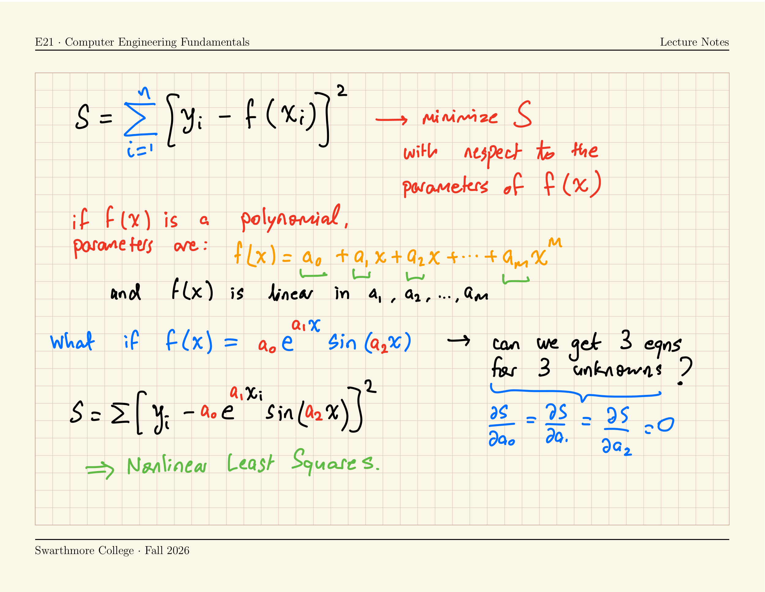
Find the parameters \(\{ a_0, a_1, a_2, ..., a_m \}\) that minimize the so-called objective function \(\boxed{S = \sum_{i} [y_i - f(x_i)]^2}\),
where \(f(x) = a_0 + a_1 x + a_2 x^2 + ... + a_m x^m\)
Note: the summation symbol refers to ‘sum over all \(n\) points’
Idea: Take derivatives with respect to \(a_0\), \(a_1\), etc. and set them all to zero, to find \(\{ a_0, a_1, a_2, ... ,a_m \}\)
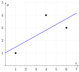
Example: a line of best fit for three points
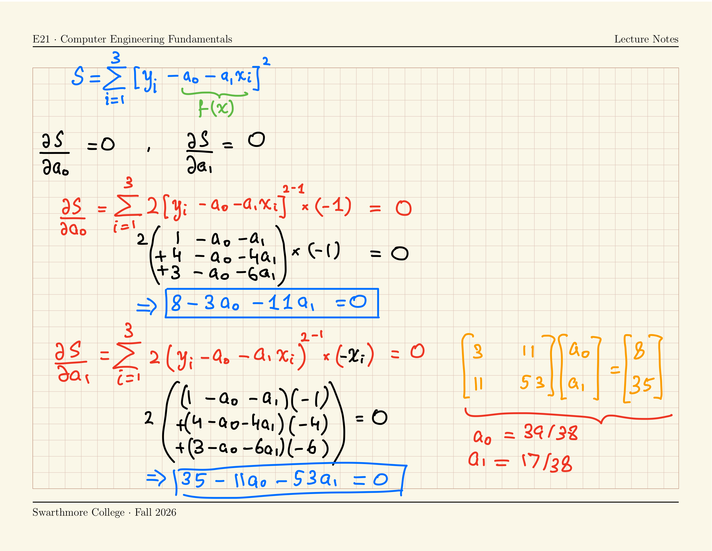
Find the equation of the straight line \(y = a_0 + a_1 x\) that passes through the three points shown while minimizing \(S\).
Hint: Write down two simultaneous equations for \(a_0\) and \(a_1\).
Solving by hand
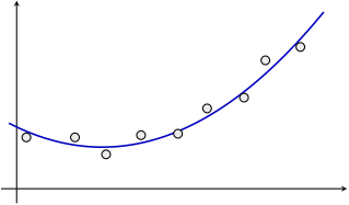
A quadratic polynomial that best fits \(n\) points
Write down the system of equations that must be solved to find the coefficients in \(y(x) = a_0 + a_1 x + a_2 x^2\).
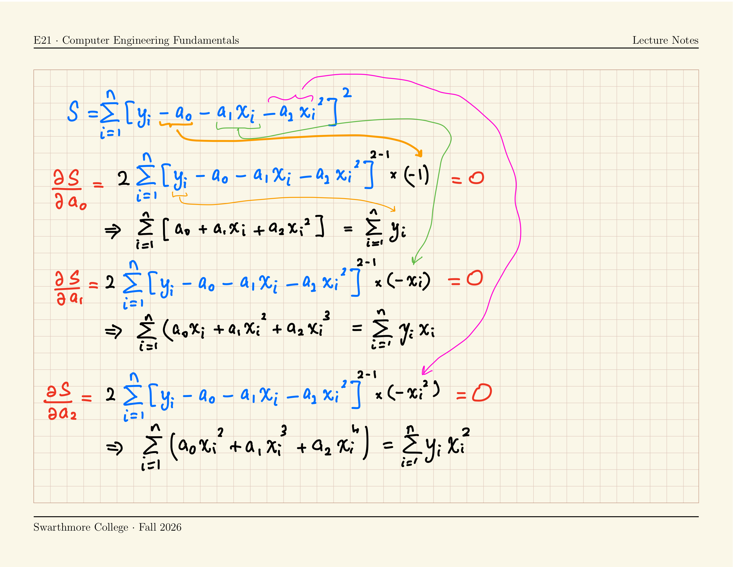
\[ \begin{aligned} \frac{\partial S}{\partial a_0} &= -2 \sum_{i} \left[ y_i - a_0 - a_1 x_i - a_2 x_i^2 \right] = 0 \\ &\implies \sum_{i} \left( a_0 + a_1 x_i + a_2 x_i^2 \right) = \sum_{i} y_i \\[1em] \frac{\partial S}{\partial a_1} &= -2 \sum_{i} x_i \left[ y_i - a_0 - a_1 x_i - a_2 x_i^2 \right] = 0 \\ &\implies \sum_{i} \left( a_0 x_i + a_1 x_i^2 + a_2 x_i^3 \right) = \sum_{i} y_i x_i \\[1em] \frac{\partial S}{\partial a_2} &= -2 \sum_{i} x_i^2 \left[ y_i - a_0 - a_1 x_i - a_2 x_i^2 \right] = 0 \\ &\implies \sum_{i} \left( a_0 x_i^2 + a_1 x_i^3 + a_2 x_i^4 \right) = \sum_{i} y_i x_i^2 \end{aligned} \]
Take derivatives \(\frac{\partial S}{\partial a_0}\), \(\frac{\partial S}{\partial a_1}\) and \(\frac{\partial S}{\partial a_2}\) and set equal to zero.
\(\displaystyle S=\sum_{i=1}^n [y_i - a_0 - a_1 x_i - a_2 x_i^2]^2\)
Derivation
System of equations for fitting a quadratic polynomial (degree \(m=2\))
\[ \begin{aligned} \sum_{i} \left( {\color{red}{a_0}}{\color{green}{x_i^0}} + {\color{red}{a_1}}{\color{green}{x_i^1}} + {\color{red}{a_2}}{\color{green}{x_i^2}} \right) &= \sum_{i} {\color{green}{y_i}}{\color{green}{x_i^0}} \\ \sum_{i} \left( {\color{red}{a_0}}{\color{green}{x_i^1}} + {\color{red}{a_1}}{\color{green}{x_i^2}} + {\color{red}{a_2}}{\color{green}{x_i^3}} \right) &= \sum_{i} {\color{green}{y_i}}{\color{green}{x_i^1}} \\ \sum_{i} \left( {\color{red}{a_0}}{\color{green}{x_i^2}} + {\color{red}{a_1}}{\color{green}{x_i^3}} + {\color{red}{a_2}}{\color{green}{x_i^4}} \right) &= \sum_{i} {\color{green}{y_i}}{\color{green}{x_i^2}} \end{aligned} \]
\[ \begin{bmatrix} \sum x_i^0 & \sum x_i^1 & \sum x_i^2 \\ \sum x_i^1 & \sum x_i^2 & \sum x_i^3 \\ \sum x_i^2 & \sum x_i^3 & \sum x_i^4 \end{bmatrix} \begin{bmatrix} a_0 \\ a_1 \\ a_2 \end{bmatrix} = \begin{bmatrix} \sum y_i x_i^0 \\ \sum y_i x_i^1 \\ \sum y_i x_i^2 \end{bmatrix} \]
Note: all sums are carried out over the \(n\) data points.
System of equations for fitting a polynomial of degree \(m\) to a set of \(n\) data points
\[ \begin{bmatrix} \sum x_i^0 & \sum x_i^1 & \sum x_i^2 & \cdots & \sum x_i^m \\ \sum x_i^1 & \sum x_i^2 & \sum x_i^3 & \cdots & \sum x_i^{m+1} \\ \sum x_i^2 & \sum x_i^3 & \sum x_i^4 & \cdots & \sum x_i^{m+2} \\ \vdots & \vdots & \vdots & \ddots & \vdots \\ \sum x_i^m & \sum x_i^{m+1} & \sum x_i^{m+2} & \cdots & \sum x_i^{m+m} \end{bmatrix} \begin{bmatrix} a_0 \\ a_1 \\ a_2 \\ \vdots \\ a_m \end{bmatrix} = \begin{bmatrix} \sum x_i^0 y_i \\ \sum x_i^1 y_i \\ \sum x_i^2 y_i \\ \vdots \\ \sum x_i^m y_i \end{bmatrix} \]
Note: all sums are carried out over the \(n\) data points.
Nonlinear Least Squares
Where \(f(x)\) depends nonlinearly on at least one of the parameters \(a_0,a_1,...,a_m\)
Linear Least Squares for functions other than polynomials
Where \(f(x)\) is a linear combination of \(m\) (possibly nonlinear) basis functions \(f_j(x)\)