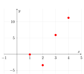
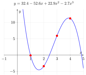
A system of \(n+1\) equations for interpolating a polynomial of degree \(n\) through \(n+1\) points on the plane
Polynomial Interpolation Matrix
Let’s look at some examples of Vandermonde matrices:
Calculate the Vandermonde matrix for for the interpolation of a cubic polynomial through the following four points: \(\begin{bmatrix} 1.0 \\ -0.1 \end{bmatrix}, \begin{bmatrix} 2.0 \\ -3.4 \end{bmatrix},\begin{bmatrix} 3.0 \\ 5.9 \end{bmatrix}, \begin{bmatrix} 4.0 \\ 11.2 \end{bmatrix}\)
def vandermonde_matrix(xlist):# Creates a Vandermonde matrix from the x-positions in `xlist` n =len(xlist) A = np.zeros((n,n),dtype=np.float64)for i,el inenumerate(xlist):for j inrange(n): A[j,i] = xlist[j]**ireturn A
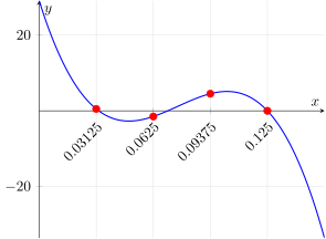
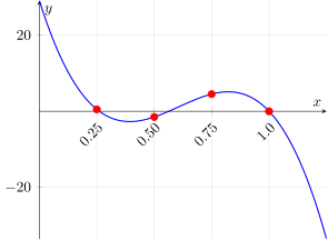
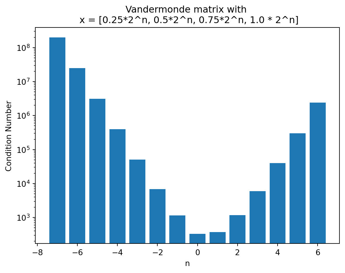
The interval over which interpolation is carried out greatly affects condition number
Condition Number versus Interpolation interval
Code
import numpy as npimport matplotlib.pyplot as pltdef vandermonde_matrix(xlist):# Creates a Vandermonde matrix from the x-positions in `xlist` n =len(xlist) A = np.zeros((n,n),dtype=np.float64)for i,el inenumerate(xlist):for j inrange(n): A[j,i] = xlist[j]**ireturn Adef vandermonde_condition_number(xlist): A = vandermonde_matrix(xlist) cond_A = np.linalg.cond(A,'fro')print(f"For a vandermonde matrix made of {xlist}")print(f"Condition number is {cond_A}")return cond_Aexponents =range(-7,7,1)output = np.zeros((len(exponents),2))for i,el inenumerate(exponents):print(f"With n = {el}") highest_number =2.0**el step_size = highest_number/4 xs = [step_size, 2*step_size, 3*step_size, highest_number] output[i,0] = el output[i,1] = vandermonde_condition_number(xs)plt.bar(output[:,0],output[:,1])plt.ylabel("Condition Number")plt.xlabel("n")plt.yscale("log")plt.title("Vandermonde matrix with \n x = [0.25*2^n, 0.5*2^n, 0.75*2^n, 1.0 * 2^n]")plt.show()
With n = -7
For a vandermonde matrix made of [0.001953125, 0.00390625, 0.005859375, 0.0078125]
Condition number is 200104475.54951715
With n = -6
For a vandermonde matrix made of [0.00390625, 0.0078125, 0.01171875, 0.015625]
Condition number is 25022246.383165702
With n = -5
For a vandermonde matrix made of [0.0078125, 0.015625, 0.0234375, 0.03125]
Condition number is 3132373.3468269915
With n = -4
For a vandermonde matrix made of [0.015625, 0.03125, 0.046875, 0.0625]
Condition number is 393841.132037466
With n = -3
For a vandermonde matrix made of [0.03125, 0.0625, 0.09375, 0.125]
Condition number is 50373.99224592936
With n = -2
For a vandermonde matrix made of [0.0625, 0.125, 0.1875, 0.25]
Condition number is 6863.662615671886
With n = -1
For a vandermonde matrix made of [0.125, 0.25, 0.375, 0.5]
Condition number is 1141.842454808791
With n = 0
For a vandermonde matrix made of [0.25, 0.5, 0.75, 1.0]
Condition number is 331.35123199279394
With n = 1
For a vandermonde matrix made of [0.5, 1.0, 1.5, 2.0]
Condition number is 371.4719547885741
With n = 2
For a vandermonde matrix made of [1.0, 2.0, 3.0, 4.0]
Condition number is 1176.9374570374491
With n = 3
For a vandermonde matrix made of [2.0, 4.0, 6.0, 8.0]
Condition number is 5956.8876457098895
With n = 4
For a vandermonde matrix made of [4.0, 8.0, 12.0, 16.0]
Condition number is 39921.7781032595
With n = 5
For a vandermonde matrix made of [8.0, 16.0, 24.0, 32.0]
Condition number is 302978.9615841781
With n = 6
For a vandermonde matrix made of [16.0, 32.0, 48.0, 64.0]
Condition number is 2390434.3340785685
Problems with Polynomial interpolation
Under certain conditions, an interpolating polynomial is guaranteed to exist mathematically.
Restrictions:
Number of points and degree of polynomial must be compatible
No two points can have the same \(y\) value
Large condition numbers cause problems
Even though the mathematical problem is typically solvable
One solution: use Newton’s method (ch.3.2 of textbook) for interpolating a polynomial
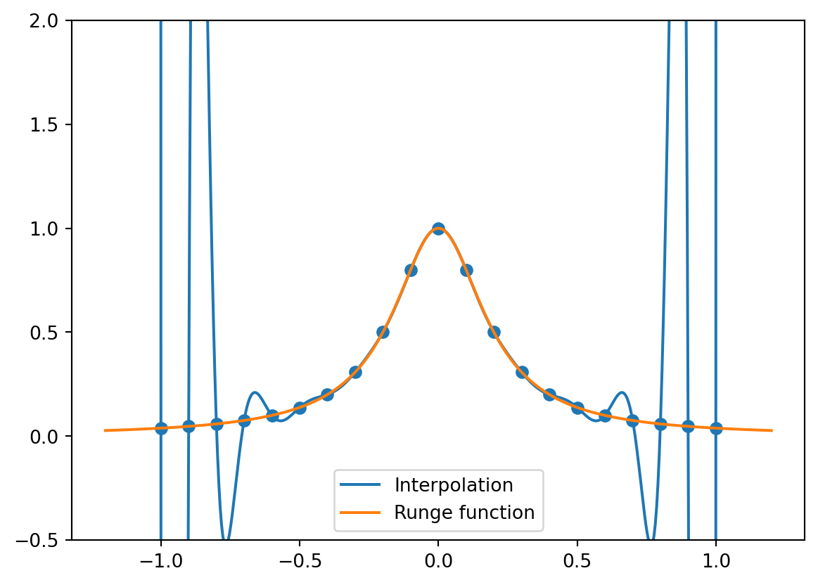
Runge’s Phenomenon
\[f(x) = \frac{1}{1+25 x^2}\]
Find an interpolating polynomial that passes through 5 equally spaced points on \(f(x)\) from \(x=-1\) to \(x=+1\)
Code
import numpy as npimport matplotlib.pyplot as pltdef vandermonde_matrix(xlist):# Creates a Vandermonde matrix from the x-positions in `xlist` n =len(xlist) A = np.zeros((n,n),dtype=np.float64)for i,el inenumerate(xlist):for j inrange(n): A[j,i] = xlist[j]**ireturn Adef Runge_func(x):return1/(1+25* x**2)def get_polynomial_coeffs(xlist,ylist):return np.dot(np.linalg.inv(vandermonde_matrix(xlist)),ylist)def evaluate_polynomial(coeffs,x): total =0for j inrange(len(coeffs)): total += coeffs[j] * x**jreturn total# Change "21" below to some other numberxvals = np.linspace(-1,1,21)yvals = Runge_func(xvals)coeffs = get_polynomial_coeffs(xvals,yvals)x_plot = np.linspace(-1.2,1.2,500)y_Runge = Runge_func(x_plot)plt.plot(x_plot,evaluate_polynomial(coeffs,x_plot),label='Interpolation')plt.plot(x_plot,Runge_func(x_plot),label='Runge function')plt.ylim([-0.5,2])plt.scatter(xvals,yvals)plt.legend()plt.show()