Problem Set 11
ENGR 12, Spring 2026.
| Due Date | Thu, Apr 16 |
| Turn in link | Gradescope |
| URL | emadmasroor.github.io/E12-S26/Homework/HW11 |
Points Distribution
Please note that each of the following grade items is a single rubric item. Each rubric item is scored on a four-level scale of 3-2-1-0. You may wish to take this into account when deciding how to allocate your efforts to each problem.
| Problem | % Weightage |
|---|---|
| Problem 1.1-1.3 | 20 |
| Problem 1.4 | 20 |
| Problem 2 | 20 |
| Problem 3.1 | 20 |
| Problem 3.2 | 20 |
1 Frequency Response of an underdamped system close to resonance
Consider a second-order system subjected to a forcing input function \[m \ddot{x} + b \dot{x} + k x = f(t) \tag{1}\] with \(m = 1, b = 2, k = 5\).
1.1 Roots
Determine the roots of the characteristic polynomial and plot them in the complex plane. Is the system stable or unstable, and underdamped or overdamped?
1.2 Fill in the following table for this system.
| Quantity | Value |
|---|---|
| \(\omega_n\) | |
| \(\zeta\) | |
| \(\omega_d\) | |
| \(\omega_r\) |
1.3 Transfer Function
Write down an expression in terms of \(s\) for the transfer function of this system. For the purpose of this transfer function, let the output be \(k x\) instead of \(x\), and let the input be \(f\) as usual, as was done in lecture 22.
1.4 Bode Plot
1.4.1 Expression for amplitude ratio
Use the expressions developed in Lecture 22 to calculate an expression for the quantitiy that will be placed on the vertical axis of the magnitude Bode plot for this system. Your expression should be in terms of only the variable \(r\), as defined in lecture.
1.4.2 Expression for phase shift
Use the expressions developed in Lecture 22 to calculate an expression for the quantitiy that will be placed on the vertical axis of the phase Bode plot for this system. Your expression should be in terms of only the variable \(r\), as defined in lecture.
1.4.3 Plot the plot
Use a computer program to make the (magnitude) Bode plot for this system, with \(0.1 < r < 10\) on the horizontal axis. Make sure to use a log-log scale for your plot.
1.4.4 Estimate low frequency and high-frequency behavior
At very high input frequencies, the system’s (magnitude) Bode plot can be approximated by a straight line on a log-log plot. The equation of this ‘straight line’ is of the form \(r^p\) where \(p\) is a number to be found. Sketch (or plot) this straight line on top of your answer to Section 1.4.3 and determine the value of \(p\).
At very low input frequencies, the system has a gain of 1. Also sketch (or plot) a straight-line approximation to this system’s Bode plot valid at these low frequencies, on top of your answer to Section 1.4.3.
2 Interpreting Bode Plots
2.1 Fourth-order
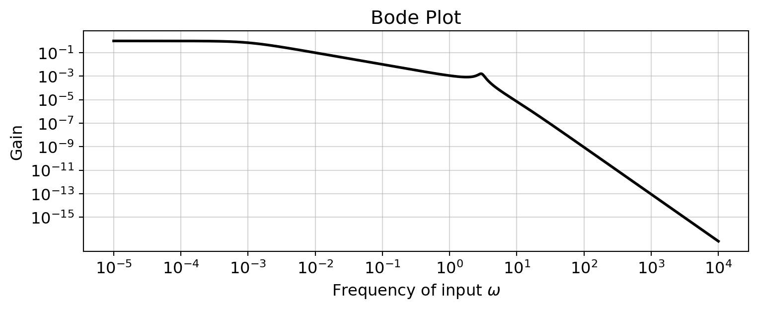
Consider the following Bode plot, which describes a system governed by the transfer function \[T(s) = \frac{9}{(s^2 + 0.6 s + 9)(0.1s+1)(1000s+1)}\]
Add a vertical line corresponding to:
- Each of the two ‘corner frequencies’ attributable to the real poles of this transfer function,
- The undamped natural frequency of this system, and
- The resonant frequency of this system.
There should be 4 lines in total.
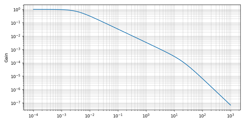
2.2 Second-order
As closely as you can, determine the transfer function whose Bode plot is shown below.
3 Another second-order system
Use the values \(m = 5, k = 10, b = 4, \omega = 4\).
Consider a second-order system subjected to a unit-amplitude sinusoidal input, \[m \ddot{x} + b \dot{x} + k x = \sin \omega t\]
The response of the system, \(x(t)\), is shown below.
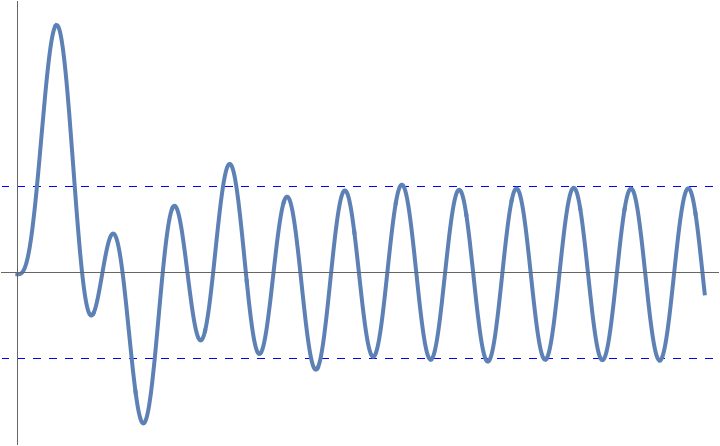
3.1 Amplitude ratio
Determine the amplitude of the sinusoidal curve in the right half of the graph above. Give your answer as a number.
3.2 Transient vs. steady-state part of the frequency response
Write down the transient part of the response of this system to the given forcing (input) function and the steady-state part of the response of this system to the given forcing (input) function.
Both parts should be functions of time involving no symbols other than the common mathematical functions and constants like \(\sin\), \(\pi\) and \(e\). Adding them up should give the graph in Figure 1.