Final Exam Solutions
ENGR 12, Spring 2026.
Solutions
1 Block Diagrams
Consider the block diagram below.
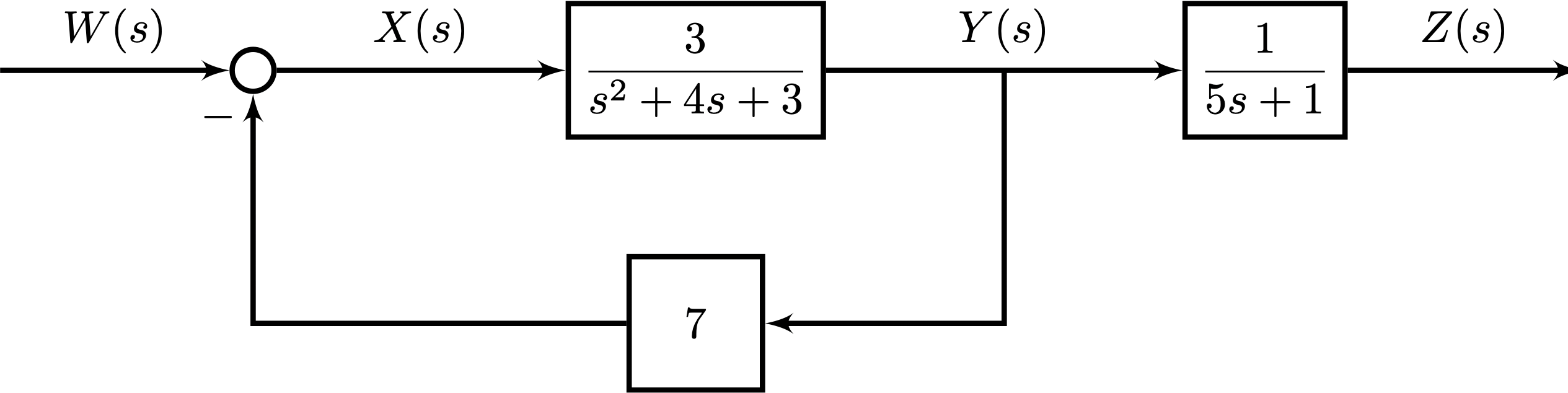
1.1 Identifying Transfer Functions by inspection
- Write down the transfer function between \(Z(s)\) and \(Y(s)\).
- Write down the transfer function between \(Y(s)\) and \(X(s)\).
- The transfer function is \[\frac{1}{5s+1}\]
- The transfer function is \[\frac{3}{s^2+4s+24}\]
1.2 Calculating Transfer Functions
Calculate the transfer function that relates the input \(W(s)\) to the output \(Y(s)\) and give your answer as a rational function (i.e., a ratio of two polynomials) in \(s\).
The summer represents the equation \(X = W - 7Y\). The block represents the equation \(Y = X \cdot \displaystyle \frac{3}{s^2+4s+3}\). Combining these two equations, we find that \[\frac{Y}{W} = \frac{3}{s^2 + 4s + 24}\]
1.3 Relating \(Z(s)\) and \(W(s)\)
Write down an equation, in terms of \(s\), that relates \(W(s)\) and \(Z(s)\). Your equation should not contain \(X(s)\) or \(Y(s)\).
Your equation need not be simplified or put into any particular form. Any correct equation relating \(Z\) to \(W\) in terms of \(s\) will suffice.
The block diagram for this system can be simplified as follows:

which suggests that the required transfer function is \[\frac{3}{s^2+4s+24} \cdot \frac{1}{5s+1}\]
for which there can be various simplifications.
1.4 The Order of a system
What is the order of the linear system shown by Figure 1 considered as a whole?
The transfer function \[\frac{3}{s^2+4s+24} \cdot \frac{1}{5s+1}\]
can be simplified as \[\frac{3}{5s^3 + 21 s^2 + 124 s + 24}\]
and this system is third order.
2 Draw Bode Plot
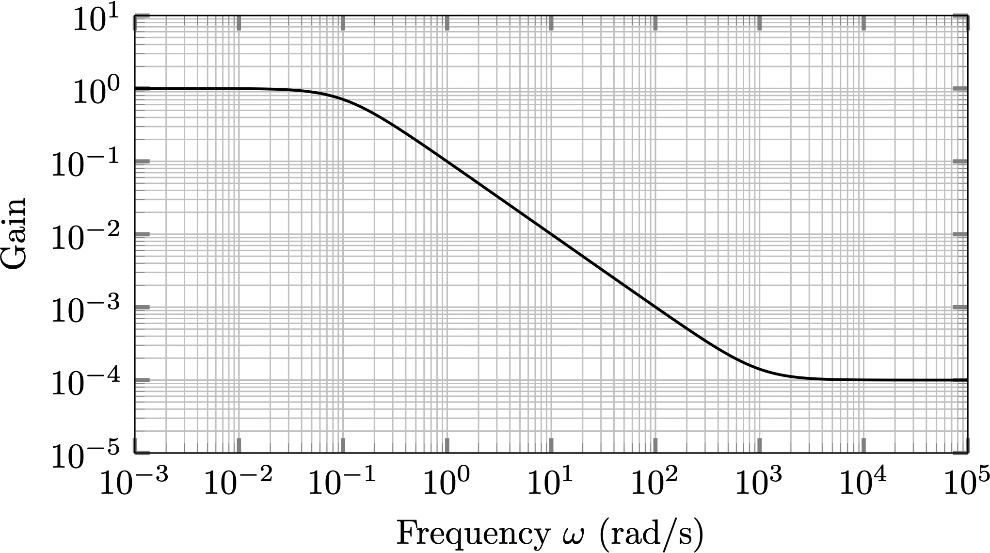
Make a qualitatively accurate sketch of the Bode plot for a system whose transfer function is \[T(s) = \frac{s/1000+1}{10s+1}\]
3 Stability
Write down either the differential equation or the transfer function for a second-order system that is unstable. Briefly show how you know that this system is unstable.
There are many ways to answer this question correctly. The essence of this question is that if a system’s characteristic equation has at least one root with positive real part, then the system is unstable. One convenient way to construct such a system is to write a transfer function of the form \[T(s) = \frac{1}{s^2 - 2 s + 3},\] which has a ‘negative damping’ term, causing its free response to exponentially grow rather than exponentially decay in magnitude.
4 Free Response of Second-order systems
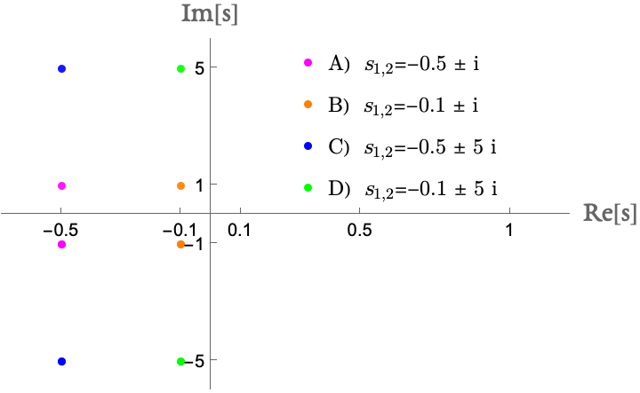
Four second-order linear systems, labeled A, B, C and D, are to be compared regarding their free response when initialized with identical initial conditions. For each system, the transfer function has exactly two complex conjugate poles given by \[s_{1,2} = r \pm i \omega_d,\] where \(r\) is the real part of the pole and \(\omega_d\) the imaginary part of the pole. The values of \(s_{1,2}\) for each system are labeled on the following diagram, which shows the real and imaginary parts of the poles of each system on the horizontal and vertical axes respectively.
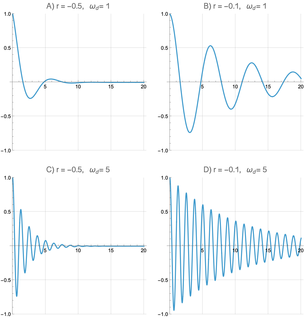
The free response of all four systems has been plotted against time in Figure 5, without labels showing which system corresponds to which graph. Label each panel of Figure 5 with letters A through D. There is only one label for each graph, and each graph has a label.
Correct labels will receive full credit. If one or more labels are incorrect, partial credit may be given for other work.
5 Spring-Mass Systems
Consider the system shown in Figure 6. A box of mass \(m\) is supported on frictionless rollers and is connected by a dashpot to the wall on the right and by a spring to a massless bar on the left, which also moves frictionlessly. The massless bar has position \(x_{\text{in}}\) and the mass has position \(x\), such that when \(x=x_{\text{in}}=0\), there is no compression or extension in the spring.
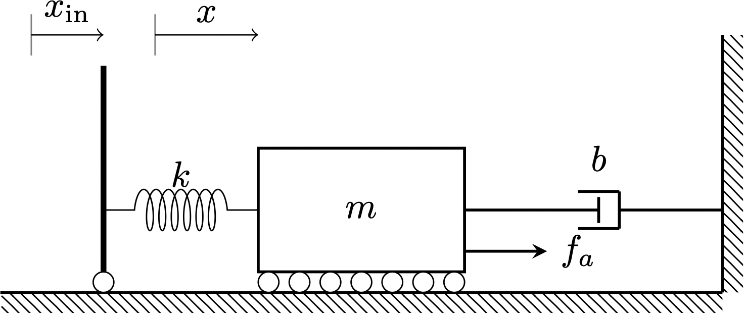
Considering the inputs to this system to be \(f_a\) and \(x_{\text{in}}\), write down the state-space equations for this system using the form \[\begin{aligned} \dot{\mathbf{x}} &= A \mathbf{x} + B \mathbf{u} \\ \mathbf{y} &= C \mathbf{x} + D \mathbf{u} \end{aligned}\] where the inputs are \(f_a\) and \(x_{\text{in}}\) and the outputs are: (1) the total compressive compressive force on mass \(m\) and (2) the distance between the massless bar and the mass \(m\).
In your answer, you should fully specify the matrices \(A\), \(B\), \(C\) and \(D\), as well as the vectors \(\mathbf{x}\), \(\mathbf{u}\) and \(\mathbf{y}\).
During the exam, it was pointed out by the instructor that the word ‘compressive’ should be crossed out from the body of the question.
The free-body diagram for the given mass is depicted below.
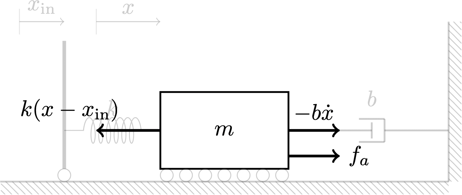
Based on this, we can write the following equation: \[m \ddot{x} = f_a - b \dot{x} - k (x - x_{\text{in}}), \tag{1}\] which can be put into the familiar form
\[m \ddot{x} + b \dot{x} + k x = f_a + k x_{\text{in}}\]
Taking the state variable to be \(\begin{bmatrix} x \\ \dot{x} \end{bmatrix}\) and the input variable to be \(\begin{bmatrix} f_a \\ x_{\text{in}} \end{bmatrix},\)
the governing equation for the state variable is
\[\frac{d}{dt}\begin{bmatrix} x \\ \dot{x} \end{bmatrix} = \begin{bmatrix} 0 & 1 \\ -k/m & -b/m \end{bmatrix} \begin{bmatrix} x \\ \dot{x} \end{bmatrix} + \begin{bmatrix} 0 & 0 \\ 1/m & k/m \end{bmatrix} \begin{bmatrix} f_a \\ x_{\text{in}}\end{bmatrix}\]
Now, the output variables of interest are the total force (taken positive to the right) on the object (let’s call this output \(y_1\)) and the distance between the object and the massless rod (let’s call this output \(y_2\)). The total force on the object is given by the right-hand side of Equation 1, which depends on the state variables as well as the inputs. The distance between the massless vertical rod and the mass is \(x - x_{\text{in}}\), which depends on a state variable and an input. Compiling the outputs into the form \(\mathbf{y} = C \mathbf{x} + D \mathbf{u}\), we can write
\[\begin{bmatrix} y_1 \\ y_2 \end{bmatrix} = \begin{bmatrix} -k & -b \\ 1 & 0 \end{bmatrix} \begin{bmatrix} x \\ \dot{x} \end{bmatrix} + \begin{bmatrix} 1 & k \\ 0 & -1 \end{bmatrix} \begin{bmatrix} f_a \\ x_{\text{in}}\end{bmatrix}\]
Thus, to summarize, we can write out the four required matrices as
\[A = \begin{bmatrix} 0 & 1 \\ -k/m & -b/m \end{bmatrix}, \quad B = \begin{bmatrix} 0 & 0 \\ 1/m & k/m \end{bmatrix}, \] \[C = \begin{bmatrix} -k & -b \\ 1 & 0 \end{bmatrix}, \quad D = \begin{bmatrix} 1 & k \\ 0 & -1 \end{bmatrix}\]
6 Impulse and Step Functions
Consider the circuit shown below.
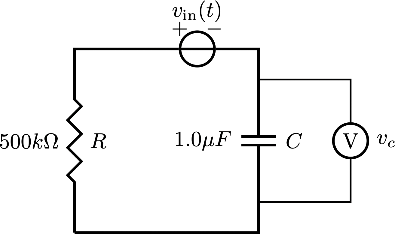
Initially, there is no energy stored in the capacitor. If the voltage source \(v_{\text{in}}(t)\) is given by the sum of the following two functions:
- A unit impulse input at time \(t=2\), and
- A unit step input starting at time \(t=4\),
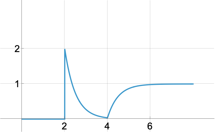
Sketch a quantitatively accurate graph of the voltage across the capacitor, \(v_c\), as a function of time, on the following axes.
7 ‘Pulse response’
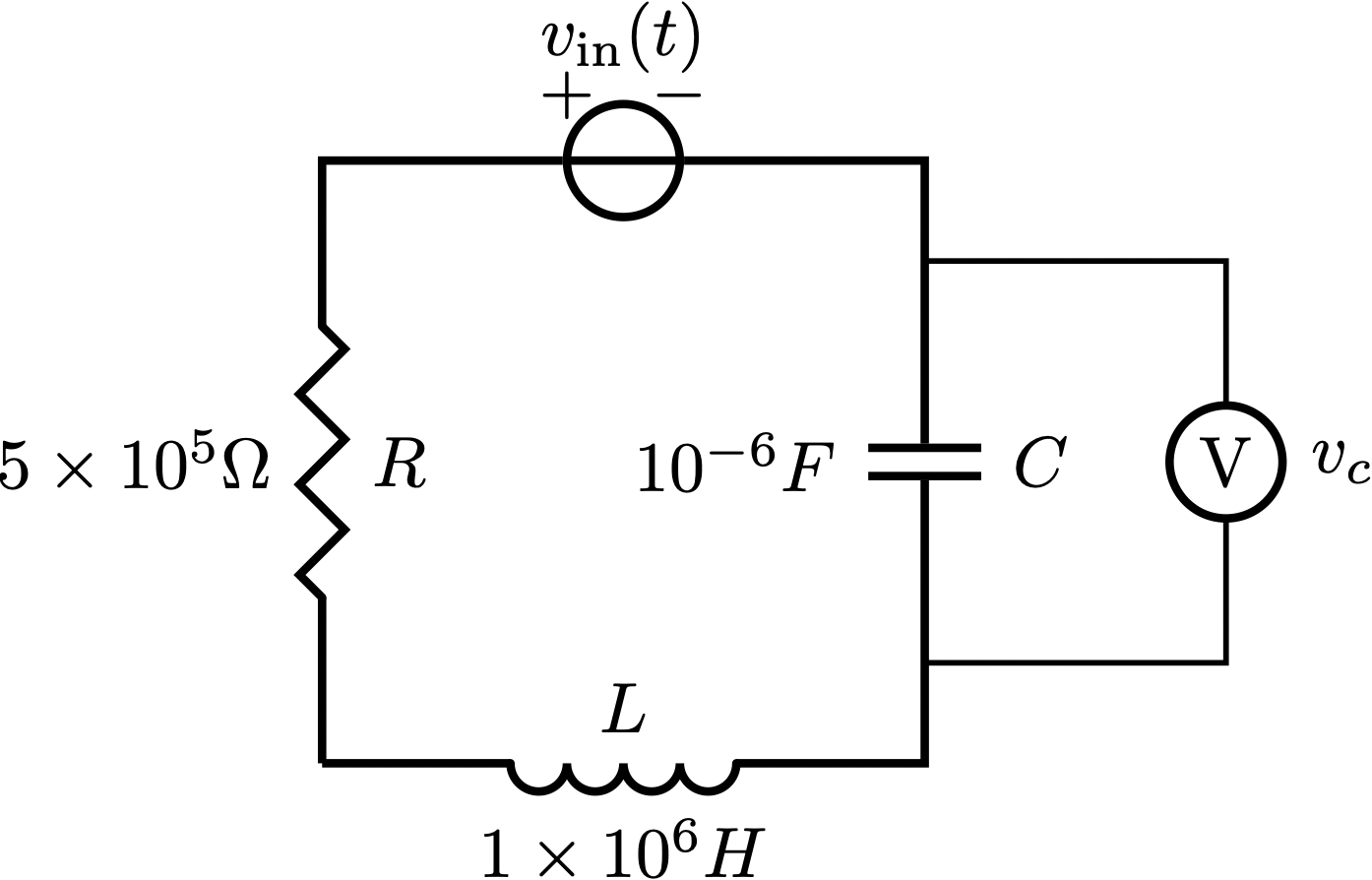
An RLC Circuit, shown in Figure 9, has a variable input voltage \(v_{\text{in}}\) given by a ‘pulse’ function \[ v_{\text{in}}(t) = \begin{cases} 0 & t < 0 \\ 2 & 0 \leq t < 20 \\ 0 & t \geq 20. \end{cases} \] It is described by the equation \(LC \ddot{v}_{c} + RC \dot{v}_c + v_c = v_{\text{in}}\)
The voltage across the capacitor is initially \(0.0\) Volts.
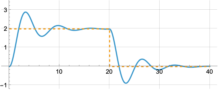
On Figure 10, sketch a qualitatively accurate graph of the voltage across the capacitor, \(v_c\), against time.
In this problem, we have \(LC = 1\) and \(RC = 1/2\) in SI units. The damping ratio \(\zeta = \frac{R \sqrt{C}}{2 \sqrt{L}}1/4\) and the time constant is \(2L/R = 4\) seconds.
8 The Fourier Transform and Bode plots
8.1 MATLAB’s fft function
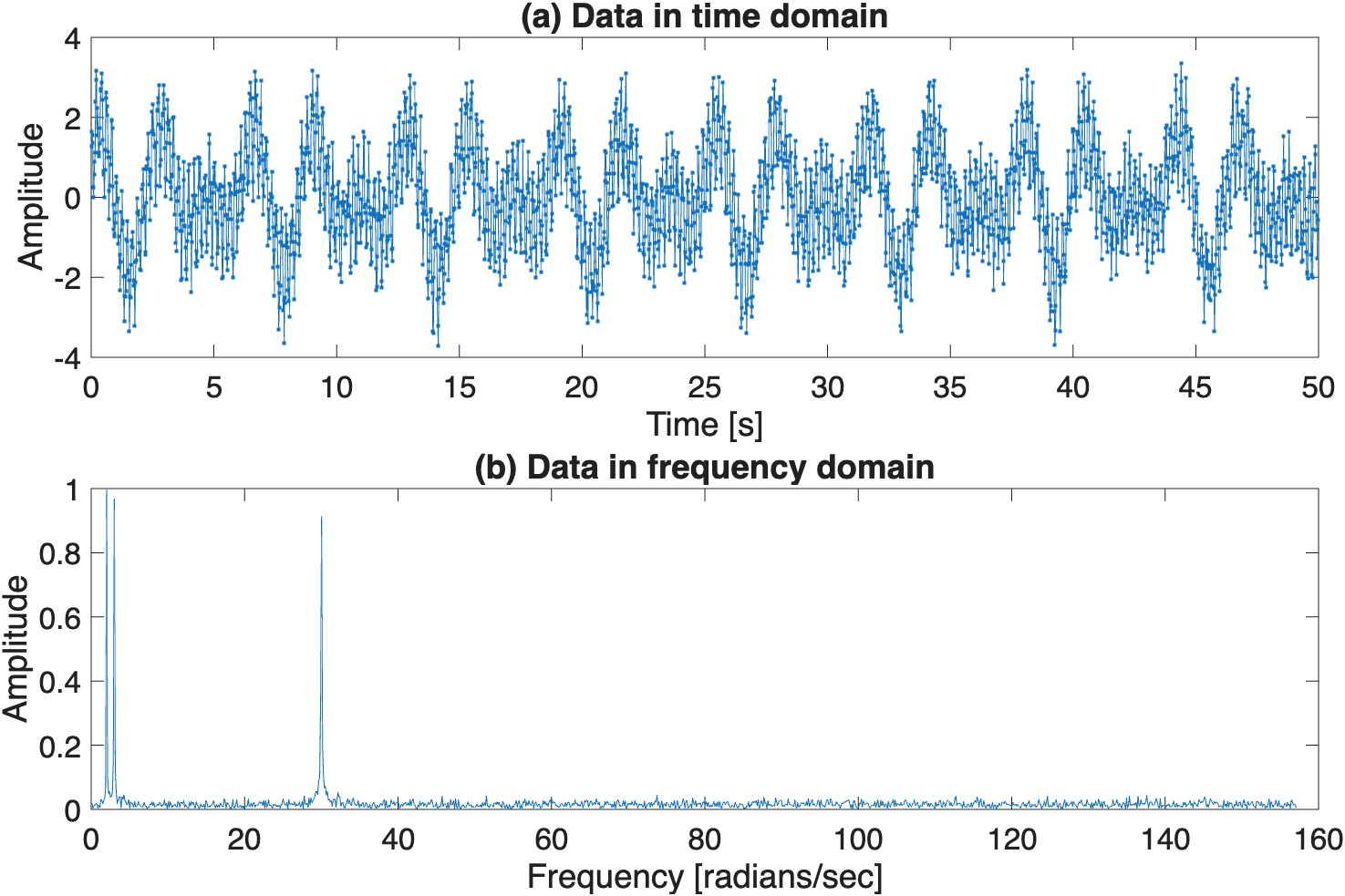
MATLAB’s fft function, which stands for ‘Fast Fourier Transform’, can be used to extract the frequency content of a signal. In Problem Set 13, we saw that fft can be used to transform data from the time domain (panel (a) of Figure 11) to the frequency domain (panel (b) of Figure 11).
Your task is to determine what the corresponding frequency-domain plot would look like if fft were used on the function shown in Figure 12. Make a sketch on Figure 13.
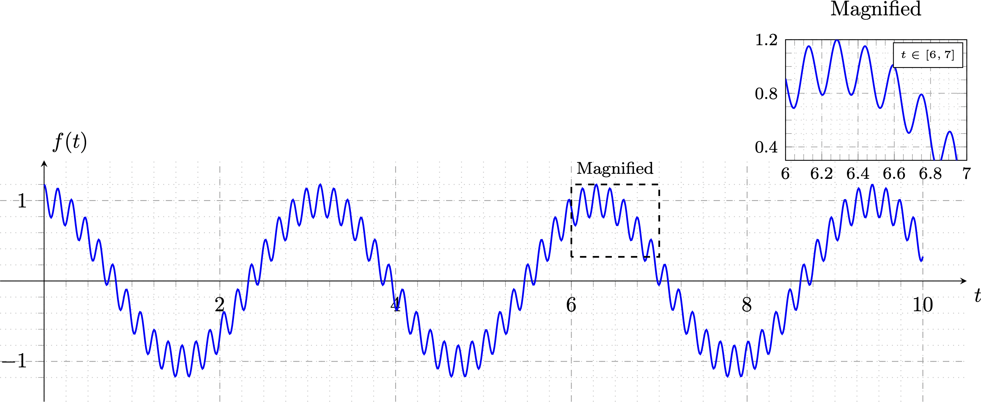
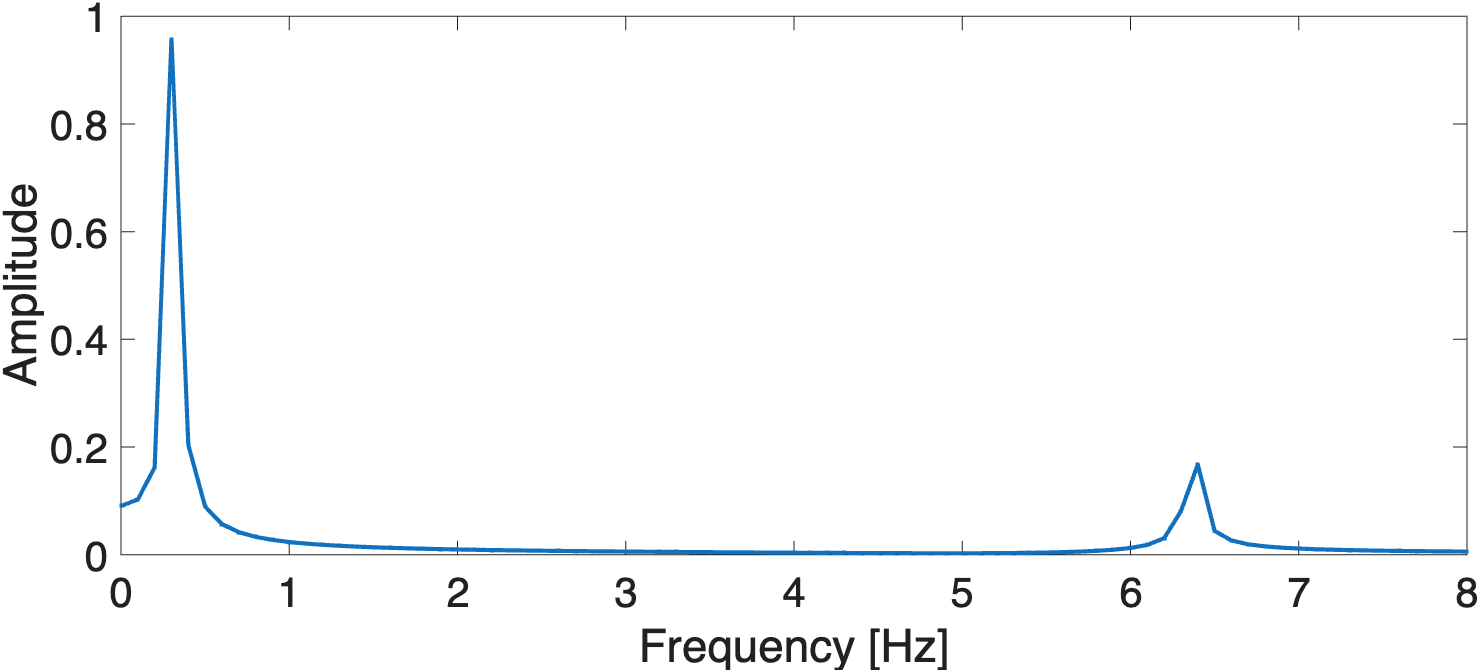
Figure 12 was produced using the following function:
\[f(t) = \cos 2t + 0.2 \cos 40 t\]
There are two constituent frequencies here:
| Property | Low-frequency signal | High-frequency signal |
|---|---|---|
| Angular frequency \(\omega\) [rad/s] | 2 | 40 |
| Frequency \(f\) [Hz] | 0.318 | 6.366 |
| Period \(T\) [seconds] | 3.142 | 0.157 |
It is possible to approximately determine these numbers by looking closely at Figure 12, where the low-frequency signal is seen to return every 3-ish seconds, and the high-frequency signal is seen to return every 0.15-ish seconds.
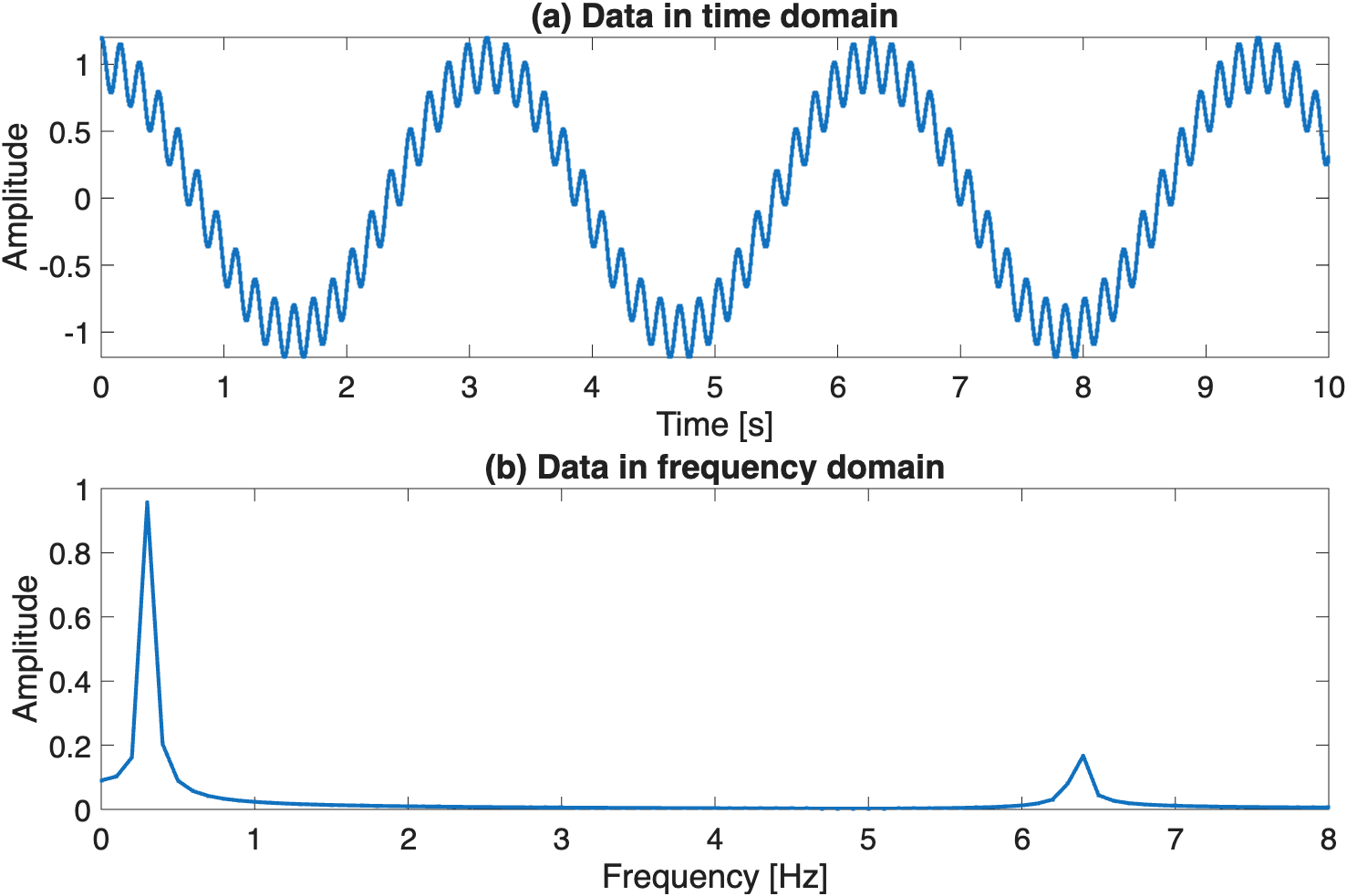
fft function to the data given in Figure 12
8.2 Bode Plot as filter
We would like to design a first-order linear system such that when the signal \(f(t)\) from Figure 12 is provided to it as input, the high-frequency signal is attennuated (i.e., reduced in amplitude) and the low-frequency signal is maintained at or near the original amplitude. Draw the Bode plot for such a first-order linear system on the axes shown in Figure 15, identify the corner frequency, and write down the transfer function associated with this linear system.
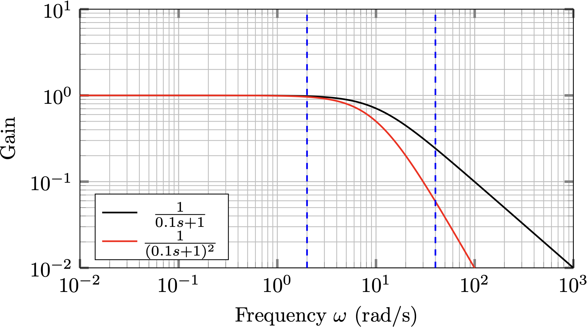
A system with transfer function such \[T(s) = \frac{1}{0.1s + 1}\] would have a Bode plot as follows. For this system, an input at an frequency of \(\omega = 2\) rad/s would have no attenuation, while an input at a frequency of \(\omega = 40\) rad/s would have significant attenuation. Other transfer functions that do the job would be acceptable as well.
Bonus: You could also construct a system with a higher-order pole, such as the one shown in red. This was not necessary for full credit.